
I know of three different ways to join together multiple tables of data. The first two are well known; use a vlookup function, and use Power Query Editor. But vlookups aren’t static calculation and can really bog down an excel document if your working with large amounts of data. If you have 10,000 rows for instance the document can start to get really bogged down. Alternatively, Power Query Editor is wonderful but somewhat new and not available on every version of excel. There is a much older version of performing a join via a query editor but its buggy, especially if you have too much data.
After some fiddling around I discovered an alternative way to splice together data using the fundamentals. This method comes in handy when the first two methods are causing issues. These days I would certain first recommend trying Power Query Editor but this is a good backup.
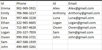
In summary, you want to make both lists the same length, then sort them by their unique identifiers, and copy the data together. It only works if their are no duplicates in either list. So this can only perform joins in a one to one relationship. In order to explain the method lets step through an example. Below are two list, one with phone numbers and the other with emails. We want to join these two tables together so we have one contact table in one place. Note that not everyone has a phone or email. For simplicity, I set names starting with “A” to only have email and names starting with “E” to only have a phone.
Step 1 – First verify that there are no duplicates in either list. If there are, you will need to remove duplicates or create a new key that’s a concatenation of multiple columns. Otherwise this method won’t work.
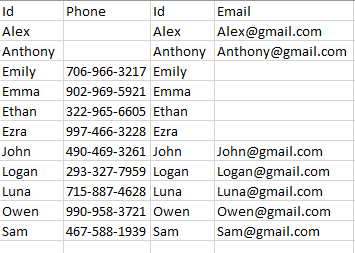
Step 2 – Copy and paste all Ids from one table to the other. Be sure to do this to both sides.

Step 3 – Remove duplicates from each table. Removing duplicates will always leave the first entry. Verify that both list are now the same length. This should leave each list with one entry for each person, regardless of which list they are on.


Step 4 – Sort both tables by Id. Be cautious here, Excel sometimes likes to sort your header along with the data, especially if you have both bodies of data in the same sheet.

Step 5 – Copy the data together. This example was done in the same sheet so I just need to remove the middle column. But everything will match up
Step 6 – Determine the type of join you want and get rid of unwanted rows. What we have done so far is create a full outer join. You will most likely want to remove one copy of the Id column as well.